AP187 Act10: Video Processing

We recorded videos showing a spinning pinwheel. Many thanks to Ma'am Jing for letting us borrow her camera. We then made the pinwheel spin by walking and running while holding it. These two instances were recorded with a camera of certain fps (frames per second). One of the videos were shown below.

Figure 1: Running with the pinwheel

The videos were parsed to obtain a set of pictures that will be color segmented. Only a part of the videos were considered; in particular, one spin of the pinwheel. Notice that there are different colored papers on the the pinwheel. These colored papers will be the region of interest (ROI) that will be used for parametric segmentation. In particular, we used the reddish paper as the ROI. Below is one of the segmented results of the parsed images from Figure 1.

Figure 2: A Segmented Image

Considering a point from the patch like in Figure 2 and considering all of the segmented images, one can trace out the spinning movement of the pinwheel. Below are the traced movements of the colored paper on the pinwheel for the walking and running instances.

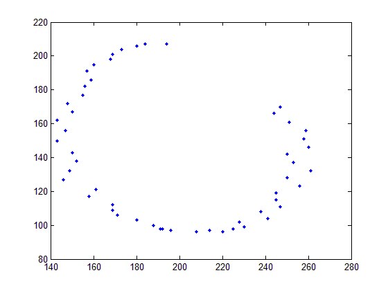
Figure 3: Path of the colored paper while running

Figure 4: Path of the colored paper while walking

One may notice that there are more data points (parsed images) for the walking instance since it will take longer for the pinwheel to complete one spin in that instance. The shapes are circular which is expected as the spinning pinwheel should trace out a circle. Some data points for the walking instance were out of the circular trend (not shown here) and can be taken into account from the choosing of a point from the patch of the segmented image.

AP187 Act9: Stereometry

In this activity, we learned the technique called stereometry in which multiple (at least two) images of different views of the same object is used to obtain depth information. Instead of using two cameras, we captured two images of the same object but one is displaced a known distance from the original.

Figure 1: Two images of a rubix cube one is displaced with respect to the other

The focus of the camera is traditionally obtained by camera calibration like in Activity 8. However, for the camera that we've used the focus is already explicitly stated to be equal to 6.6cm.

Using the equation below, we can obtain the depth of the rubix cube based on the two images.

z = bf/(x2-x1)

where,

b is the displacement between the two images
f is the focus of the camera
x2, x1 are corresponding points on the object from the two images
z is the depth of the said point

We now consider the edges of the rubix cube as the corresponding points that will be used to calculate the the depth z.

Figure 2: 3D plot of the rubix cube

The figure above was obtained by plotting the the calculated depth and its corresponding x, y coordinates from either one of the two images. The figure indeed resembles the rubix cube. Credits to BA for letting us use his camera.

AP187 Act8: Camera Calibration

We've tried different sets of inputs on a checker board. By clicking on the figures, one can see the sample points that were chosen.

The left figures shown below represent these sets of inputs. In the first set, we took sample points from the top, bottom and middle (vertical) part of the checkerboard. In the second, we considered points from the leftmost, middle and rightmost parts. In the third, sample points were taken only from the center part of the board. In the last set, we took sample points from the top, bottom and middle (horizontal) part.

Figure 1: input sample points (left) and the output of the calibration (right)

Figure 2: input sample points (left) and the output of the calibration (right)

Figure 3: input sample points (left) and the output of the calibration (right)

Figure 4: input sample points (left) and the output of the calibration (right)

As we can see, the first and fourth sets produces the best calibrations for the camera. This is seen by the red crosshairs located at the corners of the checkerboards in the right figures. Using the second set of inputs causes the calibration to fail at the top and bottom parts of the grid. While upon using the third set, the calibration fails at the outer regions of the board. This is reasonable since we only got sample points from the center.

AP187 Act5: Measuring the Gamut of Color Displays and Prints

In this activity, we determine the gamut of certain devices: a dell and an hp laptop and a projector. We displayed red, green and blue from these devices and determined their CIE xy coordinates.

Figure 1: Gamut of a dell laptop, an hp laptop, and a projector

In figure 1, the gamuts (the triangles in this case) of the devices are displayed in the CIE xy. If we compare the areas of these, the largest one would correspond to the device which can display a larger range of colors. At first glance, the gamut of the hp laptop seems to have the largest area and therefore can display a larger range of colors.

AP187 Act3: Familiarization with light-matter interaction

Figure 1: Objects demonstrating different kinds of reflection

These objects demonstrate reflection. There are three types of reflections shown here. One is specular reflection (that is, the reflection on a smooth surface). Another, body reflection, is the reflection because of the properties of the body itself. And lastly is interreflection. The reflection because of this is because of light coming from another object.

Figure 2: Objects demonstrating diffraction

Light may scatter when it interacts with matter. This scattering will be dependent on the wavelength of the incident light. So for certain materials, it will cause light to separate into different colors. Due to the wave nature of light when it reaches an aperture, light gets diffracted and casts a shadow shown in the picture.

Figure 3: Example of transmission and absorption

As seen from the picture, the image through the piece of glass is different. This is because this glass absorbs and transmits certain wavelengths of light.

Figure 4: Color addition and subtraction

Trichromaticity and addition and subtraction of color are demonstrated in these pictures.

Reflectances

Below are the reflectances from different colored objects.

Figure 5: Reflectance spectrum of a blue colored notebook

Figure 6: Reflectance spectrum of a blue colored notebook with checkered patterns

Figure 7: Reflectance spectrum of a green colored notebook

Figure 8: Reflectance spectrum of an orange colored umbrella

Figure 9: Reflectance spectrum of the cast of the orange colored umbrella

Figure 10: Reflectance spectrum of peach colored notebook

Figure 11: Reflectance spectrum of pink colored notebook

Figure 12: Reflectance spectrum of yellow colored notebook

AP187 Act2: Familiarization with Properties of Light Sources

In this activity, we gained knowledge on the properties of different light sources.

We gathered the following light sources: 2 cellphone LCDs, incandescent light, stove, flourescent and sunlight. The emittance spectra of the said light sources were then obtained using a spectroradiometer. Results are shown below.

Emittance Spectra of two Cellphones

The spectra from the two cellphone displays are very similar. They have "peaks" in the reddish and greenish regions.

Emittance Spectra of a Flourescent Lamp

In the spectra, there are several distinct peaks. This may be the remnants of the spectrum of the elements inside the flourescent lamp.

Emittance Spectra of a Incandescent Lamp

This particular emittance suggest that the incandescent lamp is "broadband". That is, its spectra is made up of a large number of wavelengths as opposed to monochromatic light which only has one wavelength.

Emittance Spectra of a Stove

At high enough temperatures, a heated object will emit light. This spectra is from a heated stove. It is hard to interpret it since the peaks may represent noise.

Emittance Spectra of a Sunlight

The spectra of sunlight is also broadband since it is the combination visible light. However, the graph suggest that it contains more reddish-greenish light than blue light.

Next, we computed for the emittance spectrum of a blackbody radiator for temperatures in the range. A video below shows how the emittance spectrum varies as the temperature increases. With this, we will be able to identify the color that an object will emit given its temperature.